RAMP: predicting the neural origin of magnetic signals
Paris Saclay Center for Data Science (Inria)
|
|
Table of contents
Note: If you are having issues with rendering of this notebook (eg the mathematical formulas are not displaying correctly) please view it on nbviewer.
Introduction 
Brain activity produces electrical currents which generate electromagnetic fields. Both electric and magnetic signals resulting from brain activity can be recorded from the scalp of subjects with the help of electroencephalography (EEG) and magnetoencephalography (MEG) respectively.
In this challenge, we will focus on the magnetic signals recorded by MEG. Your aim will be to estimate a model that can predict which brain areas are at the origin of the measured MEG signal. This challenge is based on realistic simulations in order to have access to the ground truth and quantitatively evaluate the performance of the models.
Origin of electrical signals in the brain 
Communication between brain cells (neurons) happens at synapses. That's where the signal is passed from one neuron to another, causing an electrical current to flow within and outside the neuron. A current flowing into one part of the neuron (forming a current sink) flows within the neuron and must leave it elsewhere (forming a current source). The source and sink pair forms a current dipole. The dipole generated by a single neuron can be therefore understood as a vector with constantly changing direction and length.
Below you can see a visualization of a positive current (excitatory synaptic input) entering at different locations of 4 neurons. The background color represents the strength of the electric field, the color bar is in nV. Please note, that in real conditions there are many such inputs happening simultaneously.
|
A schema of 4 neurons with the same morphology. Each is stimulated with the synaptic input at different locations (red dot) but at the same time. This is where the current enters the cell. Then, most of it flows through the cell and comes out of the cell body (purple dot) forming a dipole. The direction and relative size of the dipole of each cell is represented by a purple line. Note the differences between the 4 neurons. The colors in the background show the changes in the extracellular electric field. |
Origin of magnetic signals in the brain 
So far we have only talked about the electric currents, but you might remember from your physics class that electrical currents are always associated with a magnetic field. This has been understood since the discovery of Maxwell's equations. Now, if you consider the electrical currents and the dipoles which we discussed above, you can imagine magnetic fields forming closed loops around them.
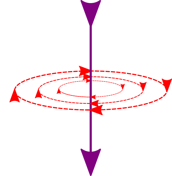
|
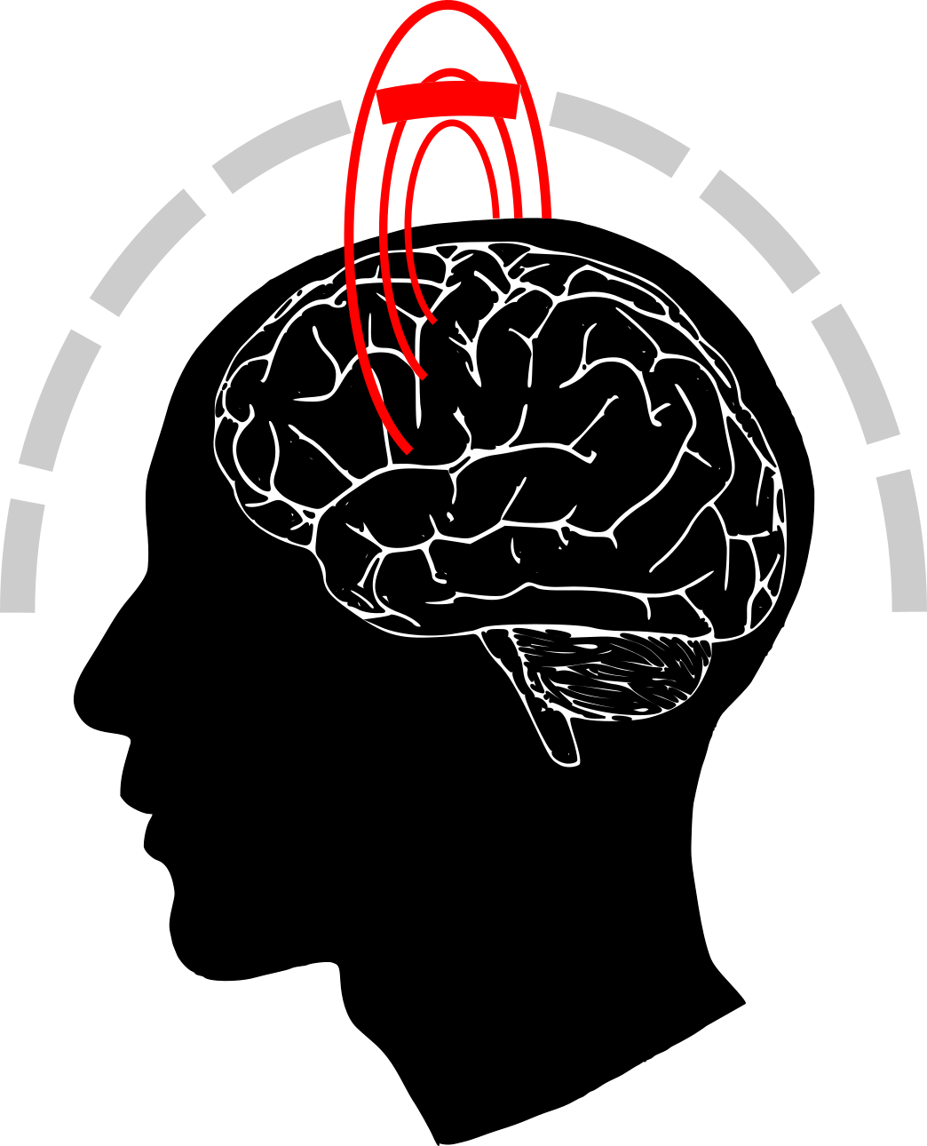
The current flow is represented by the purple line (left), and the red lines show the direction of the magnetic field. Those magnetic fields are then recorded by the MEG sensors (grey on the right). |
|
Neurons are constantly active, constantly receiving and propagating electrical signals, but a single neuron is relatively tiny and therefore the potential it generates is too small to be recorded from the scalp. However, there are billions of neurons in the human brain which together form brain structures. Many of the neuron types align and correlate. As you can imagine, in this environment some of the single-cell dipoles are cancelled out while the others add up to form a much stronger signal. This group signal (from the single-cell dipoles that add up) along with a lot of noise can be recorded by MEG or EEG.
Keep in mind that due to the alignment of cell bodies in the brain, it is the magnetic fields generated by the intracellular current (i.e. current flowing inside the cell) that generate the signals recorded by MEG, whereas the transmembrane currents (flowing inside/outside the cell) are responsible for EEG signals.
Please note that this is only a simplified explanation.

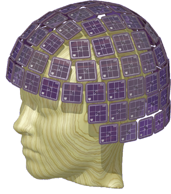
|
An actual MEG measurement system (left). It's a VectorView system produced by the MEGIN company. Such a system contains 306 MEG sensors (right). Each of the 102 blue square contains 3 MEG sensors. |
|
MEG in practice and problem description
There are a lot of things happening in the human brain at every moment, so how is it possible to know which signals to look for? The subject participating in a cognitive neuroscience experiment is usually asked to perform the same task multiple times (watching something on a screen, remembering something, pressing buttons etc.). Then the recorded signals obtained during all the repetitions of the experiment are averaged, leading to noise reduction and cleaner data related to that task. This is related to so-called evoked responses. However, a major challenge facing the neuroscientists is to figure out where exactly the signal is coming from. Solving this problem is known as 'MEG source imaging', 'source localization' or 'electromagnetic brain mapping'. See for example Baillet et al. 200 Mosher et al. 1999 Becker et al. (2015) or this article on scholarpedia.
Mathematical foundations of MEG source imaging
If one denotes by $x \in \mathbb{R}^p$ the MEG data at one time point, where $p$ is the number of sensors, one has that $x$ is obtained from a linear combination of sources. The linearity is a fact derived from the linearity of Maxwell equations. Assuming the sources can originate from a finite set of $q$ locations in the brain, one has that the data $x$ is related to the source amplitudes $z \in \mathbb{R}^q$ via a matrix $L$ of size $p \times q$, known as the 'lead field matrix', the 'gain' or 'forward operator'. It represents the sensitivity of each sensor to signals from each source location. For example, if the value of $L_{i,j}$ is high, it means that a signal from the $j^{th}$ source with amplitude $z_j$ would result in a high measurement in the $i^{th}$ sensor, i.e. a strong coefficient $x_i$. Conversely, if the value of $L_{i,j}$ is close to 0, it means that a signal from the $j^{th}$ source would result in a very weak measurement in the $i^{th}$ sensor.
Assuming the presence of some additive noise $n \in \mathbb{R}^p$ it leads to: $$ x = Lz + n \enspace . $$
This is a linear regression model, and $z$ corresponds to the regression coefficients.
Solving the source imaging problem, i.e. estimating $z$ from $x$, is the question we ask of you in this challenge: given some simulated MEG data you should predict the brain region(s) (sources) where those signals originate from. We have simulated the MEG data in this challenge as this allows us to know the 'ground truth' source location(s). Each simulation consists of signals generated from one or more sources, which are randomly selected.
First, let's explore the data.
Data exploration 
Import 
Prerequisites
- Python >= 3.7
- numpy
- scipy
- osfclient
- pandas
- pot
- imbalanced-learn
- scikit-learn
- matplolib
- jupyter
- ramp-workflow
- ramp-utils
The following cell will install the required pacakge dependencies, if necessary.
import sys
!{sys.executable} -m pip install scikit-learn
!{sys.executable} -m pip install ramp-workflow
!{sys.executable} -m pip install ramp-utils
To get this notebook running and test your models locally using ramp-test (from ramp-workflow), we recommend that you use the Anaconda or Miniconda Python distribution.
import numpy as np
import matplotlib.pyplot as plt
import pandas as pd
from scipy import sparse
import os
Download the data (optional) 
If the data has not yet been downloaded locally, uncomment the following cell and run it. Be patient. This may take a few minutes. The download size is less than 150 MB.
# !python download_data.py
You should now be able to find the test and train folders in the data/ directory
MEG recordings 
To load the data we will be using the function called get_train_data() and/or 'get_test_data()' defined in problem.py. RAMP is also using those functions:
from problem import get_train_data, get_test_data
X_train, y_train = get_train_data()
X_train.columns
The data has a lot of columns named e1, e2, ... , e204 column named 'subject' and 'L_path'. Each column marked with 'e' is the recording from one of the MEG sensors. We have used 204 sensors for the MEG recordings. It corresponds to the gradiometers in a VectorView system (the other 102 are magnetometers that are ignored here for simplicity). Each row represents the signal from all 204 sensors at one timepoint for one simulation. Recall that each simulation consists of signals generated from one or more sources, which are randomly selected.
'subject' is the subject ID of the participant on whom this recording was performed.
'L_path' is a path to an additional data for each subject (lead_field) which we will discuss later.
Let's see what subjects we have:
np.unique(X_train['subject'])
X_train.shape
The number of subjects is much smaller than the number of rows because there is a large number of simulations for each subject.
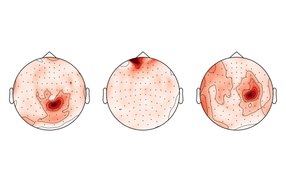
Let's now look at the heat maps on the head of the first three samples:
(optional) If you wish to see and run the code that plots the above heatmaps, you will have to additionally install the MNE-Python library and uncomment the following line and run it:
# %load plot_topomap.py
The above heatmaps are taken from the first three samples of the train dataset. The darker the color, the higher is the recorded value.
Can you already make a guess how many brain sources lead to the generation of these signals?
Before we look at the ground truth let's discuss what we actually mean by 'source'. The brain is a continuous mass and so we could consider millions of points (individual neurons) to be a potential source. Classically for MEG/EEG source imaging the cortex is discretized. This is illustrated in the following figure where every yellow code is the potential location of a source. Here you see about 4000 locations sampled over the left hemisphere. With two hemispheres it leads to about 8000 locations, meaning that one assumes that $q \approx 8000$. Remember that we have $z \in \mathbb{R}^q$.
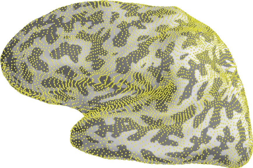
While recovering $z$ from $x$ is the ultimate objective of source imaging, $q$ being much larger than $p$ makes this problem really hard. The problem is 'ill-posed'. To simplify the task for the sake of this challenge, we subdivided the brain of each subject into 450 subregions; their technical name is 'parcels' (225 parcels per hemisphere, the corpus callosum, located between the two hemispheres, is excluded). Each parcel is a part of a larger region which has an anatomical meaning (represented by different colors below):
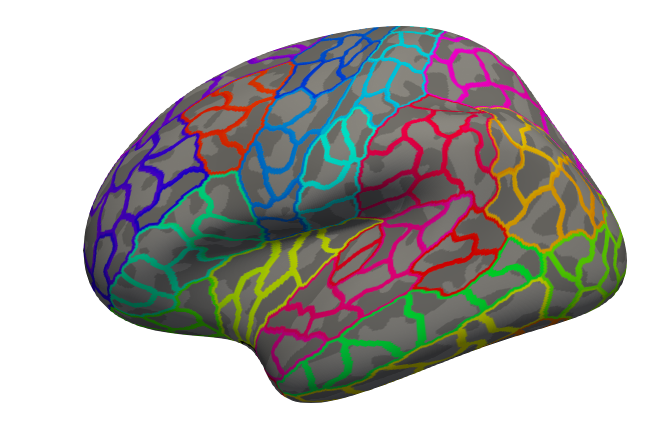
Your task is to predict which parcel(s) the MEG signal originates from. So let's look at the target:
print(y_train)
What you can see is an array mostly filled with 0s. Each column represents one of the 450 brain parcels. A 1
indicates the source of the signal comes from that brain parcel. Each row in the data represents one sample. You can see this problem in machine learning sense as a multioutput binary classification problem (predict if each parcel is active or not) or also as a multi-label classification problem as your task boils down to the prediction of a list of active parcels.
You should be able to guess what the shape of the target is, can you?
print(f'There are {y_train.shape[0]} samples and {y_train.shape[1]} brain parcels')
And let's see if you guessed correctly the number of sources in each of the three heatmaps above!
n_sources_per_sample = np.sum(y_train, axis=1)
print(f'Number of sources in first three samples: {n_sources_per_sample[:3]}')
Because we simulated this data (using the MNE-Python library) we were free to limit the number of sources. Let's check the possible number of sources, in all our samples:
n_sources_per_sample = np.sum(y_train, axis=1)
n_possible_sources = np.unique(n_sources_per_sample)
print(f'Possible number of sources: {n_possible_sources}')
k-nearest neighbors algorithm 
We are now going to make some predictions. We will start from the algorithm called k-nearest neighbors. You can read more about it in the Wikipedia or scikit-learn documentation.
Let's also look at the 'test' dataset:
X_test, y_test = get_test_data()

# print info
print(f"There are {len(X_train)} measurements"
      f" recorded from {len(np.unique(X_train['subject']))} subjects"
      " in the train dataset, and\n"
      f"{len(X_test)} measurements"
      f" recorded from {len(np.unique(X_test['subject']))} subjects"
      " in the test dataset.")
To decrease calculation time from now on we will only work on the subset of the data but feel free to use the full dataset
def decrease_data_size(X, y):
    # decrease datasize
    X = X.reset_index(drop=True)  # make sure the indices are ordered
    # 1. take only first 2 subjects
    subjects_used = np.unique(X['subject'])[:2]
    X = X.loc[X['subject'].isin(subjects_used)]

    # 2. take only n_samples from each of the subjects
    n_samples = 100  # use only 100 samples/subject
    X = X.groupby('subject').apply(
        lambda s: s.sample(n_samples, random_state=42))
    X = X.reset_index(level=0, drop=True)  # drop subject index

    # get y corresponding to chosen X
    y = y[X.index]

    return X, y

X_train, y_train = decrease_data_size(X_train, y_train)
X_test, y_test = decrease_data_size(X_test, y_test)
First, import all the libraries which we will need:
from sklearn.compose import make_column_transformer
from sklearn.multioutput import MultiOutputClassifier
from sklearn.neighbors import KNeighborsClassifier
from sklearn.pipeline import Pipeline
Let's instantiate a KNeigborsClassifier:
# K Nearest Neihbors
clf = KNeighborsClassifier(n_neighbors=3)
If we just use KNeigborsClassifier on our data it will not work because the target is multioutput, meaning that we may have more than a single predicted output. That is why we also use MultiOutputClassifier, which takes the KNeighborsClassifier we just created as an input:
kneighbors = MultiOutputClassifier(clf)
However, what we have done so far is not yet sufficient. Because the data X not only consists of the sensor measurements (dtype: float64) but also of the 'subject' ID and the 'L_path' which are of dtype: object:
X_train.dtypes
KNeighbors won't accept this data type. Here, we decide to just drop the whole 'subject' and 'L_path' columns and do not use the information about the subjects. We can do it using ColumnTranformer or the function make_column_transformer:
preprocessor = make_column_transformer(('drop', ['subject', 'L_path']),
                                       remainder='passthrough')
Now, we can create a scikit-learn pipeline that first drops the column, and then makes use of our multi-output k-nearest-neighbors classifier.
Note: RAMP submissions must consist of a function that returns a scikit-learn pipeline.
pipeline = Pipeline([
        ('transformer', preprocessor),
        ('classifier', kneighbors)
    ])
The code presented above is implemented as a sample solution in: submissions/starting_kit/estimator.py. If you wish to load it here, uncomment the line below:
# %load submissions/starting_kit/estimator.py
Let's fit this pipeline with the data and make a prediction.
For now we will use the Jaccard error (meaning [1-jaccard score]), but please refer to Performance metric section for the details of the scores based on which you are going to be evaluated.
pipeline.fit(X_train, y_train)
y_pred_knn = pipeline.predict(X_test)
from sklearn.metrics import jaccard_score

score_knn = 1 - jaccard_score(y_test, y_pred_knn, average='samples')
print(f"The jaccard error for KNN is {score_knn}")
n_sources_per_sample = np.sum(y_pred_knn, axis = 1)
n_sources = np.unique(n_sources_per_sample)
print(f'Predicted number of sources: {n_sources}')
Lead fields 
Looking at your data files you probably realized that there are more files than just X.csv and target.npz for 'test' and 'train' in your data folder. You also have some files stored in data/ directory. Their names begin with a subject id and end with "_L.npz" (e.g. subject_1_L.npz or subject_2_L.npz etc.). As we said earlier in your data X one of the columns called L_path corresponds to the paths of those files (note that although we store the path in each row of X esentially for each given subject there is a single lead_field file. These files contain the lead field matrices $L \in \mathbb{R}^{p \times q}$ for each of the subjects. Perhaps you have noticed that the id corresponds to the id of the subject in your X.csv data file. Let's load one file to see what it contains:
path_subject_1 = X_train[X_train['subject'] == 'subject_1']['L_path'].iloc[0]
print('first path is: ', path_subject_1)
lead_field = np.load(path_subject_1)
L = lead_field['lead_field']
L.shape
Each brain is different in shape and structure. Therefore, the signal propagates differently from the source to the sensors in each subject. You have therefore a different lead field for each subject.
Again 204 is the number of MEG sensors and 4688 is the number of possible brain locations (yellow dots above). Note that this is not the number of brain parcels - 450.
As we mentioned previously, each brain parcel we consider is a specific 'subregion' in the brain. Each brain parcel is made up of a number of possible locations. The source can be single location within a parcel. The number of locations that make up each parcel varies between subjects (a given parcel can have a different extent for each subject). This information is stored in 'lead_field'. The parcel index that corresponds to any location for a subject is stored in 'lead_field' file.
Let's look at the 'lead_field' of another subject:
path_subject_2 = X_train[X_train['subject'] == 'subject_2']['L_path'].iloc[0]
lead_field = np.load(path_subject_2)
lead_field['lead_field'].shape
Notice above that the number of columns is different from the first 'lead_field' file. This is because, as stated above, the number of locations for each subject can vary a bit.
lead_field['lead_field'] is of shape (n_sensors, n_locations).
So how do we match which location belongs to which parcel? In your 'lead_field' file you will find another argument called parcel_indices:
parcel_indices = lead_field['parcel_indices']
print(parcel_indices.shape)
parcel_indices[:10] # let's look at the index of the first 10 locations
print(f"There are {len(parcel_indices)} values each of which can be one of "
      f"{len(np.unique(parcel_indices))} unique numbers, which correspond to the 450 parcels.")
Each number in parcel_indices tells us which parcel each point belongs to. The 450 parcel numbers correspond to the parcels represented by the 450 columns in the target y.
How can we use this information for the predictions?
Lasso algorithm 
We will now construct slightly more complicated estimator which will use 'lead_fields' (later also called '$L$'). First we want to load the 'lead_fields' which are used in our data.
Remark: Note that we are scaling all the 'lead_fields' by 1e8 in the get_leadfields function. That is to avoid having too small numbers given to the estimator.
The idea of the Lasso is to estimate $z \in \mathbb{R}^q$ as:
$ \hat{z} \in \mathop{\mathrm{arg\,min}}_z \frac{1}{2p} \| x - Lz \|_2^2 + \alpha \|z\|_1 $
Due to the $\ell_1$ norm such a strategy leads to a sparse solution, i.e. many entries in $\hat{z}$ will be 0. We will then look at the non-zero entries in $\hat{z}$ to know if a parcel is active or not. The higher is $\alpha$ the less number of active parcels you will estimate. If $\alpha$ is too high you will then predict that no parcel is active. You can refer to the wikipedia page on Lasso or this example on the scikit-learn website.
Now we will write a class SparseRegressor which will accept an estimator (i.e. model) that solves the inverse problem, i.e. estimating $z$ (in the code below called est_coef) from $x$ and $L$. Such an estimator is a regressor whose estimated coefficients allow to predict which parcel is active. Note we now use the individual leadfield matrices.
from sklearn.base import BaseEstimator, ClassifierMixin
from sklearn.base import TransformerMixin


def _get_coef(est):
    """Get coefficients from a fitted regression estimator."""
    if hasattr(est, 'steps'):
        return est.steps[-1][1].coef_
    return est.coef_


class SparseRegressor(BaseEstimator, ClassifierMixin, TransformerMixin):
    '''Provided regression estimator (ie model) solves inverse problem
        using data X and lead field L. The estimated coefficients (est_coef
        sometimes called z) are then used to predict which parcels are active.

        X must be of a specific structure with a column name 'subject' and
        'L_path' which gives the path to lead_field files for each subject
    '''
    def __init__(self, model, n_jobs=1):
        self.model = model
        self.n_jobs = n_jobs
        self.parcel_indices = {}
        self.Ls = {}

    def fit(self, X, y):
        return self

    def predict(self, X):
        return (self.decision_function(X) > 0).astype(int)

    def _run_model(self, model, L, X):
        norms = np.linalg.norm(L, axis=0)
        L = L / norms[None, :]

        est_coefs = np.empty((X.shape[0], L.shape[1]))
        for idx, idx_used in enumerate(X.index.values):
            x = X.iloc[idx].values
            model.fit(L, x)
            est_coef = np.abs(_get_coef(model))
            est_coef /= norms
            est_coefs[idx] = est_coef

        return est_coefs.T

    def decision_function(self, X):
        X = X.reset_index(drop=True)

        for subject_id in np.unique(X['subject']):
            if subject_id not in self.Ls:
                # load corresponding L if it's not already in
                L_used = X[X['subject'] == subject_id]['L_path'].iloc[0]
                lead_field = np.load(L_used)
                self.parcel_indices[subject_id] = lead_field['parcel_indices']

                # scale L to avoid tiny numbers
                self.Ls[subject_id] = 1e8 * lead_field['lead_field']
                assert (self.parcel_indices[subject_id].shape[0] ==
                        self.Ls[subject_id].shape[1])

        n_parcels = np.max([np.max(s) for s in self.parcel_indices.values()])
        betas = np.empty((len(X), n_parcels))
        for subj_idx in np.unique(X['subject']):
            L_used = self.Ls[subj_idx]

            X_used = X[X['subject'] == subj_idx]
            X_used = X_used.drop(['subject', 'L_path'], axis=1)

            est_coef = self._run_model(self.model, L_used, X_used)

            beta = pd.DataFrame(
                np.abs(est_coef)
            ).groupby(self.parcel_indices[subj_idx]).max().transpose()
            betas[X['subject'] == subj_idx] = np.array(beta)
        return betas
from sklearn import linear_model

model_lars = linear_model.LassoLars(alpha=1.0, max_iter=3,
                                    normalize=False,
                                    fit_intercept=False)

lasso_lars = SparseRegressor(model_lars)
lasso_lars.fit(X_train, y_train)
y_pred_lassolars = lasso_lars.predict(X_test)
score_lassolars = 1 - jaccard_score(y_test, y_pred_lassolars, average='samples')
print(f'Jaccard error for the Lasso Lars algorithm using lead fields is {score_lassolars}')
The score is very bad. Let's see how well the number of sources is predicted:
n_sources_by_sample = np.sum(y_pred_lassolars, axis = 1)
n_sources = np.unique(n_sources_by_sample)
print(f'Predicted possible number of sources: {n_sources}')
So in fact, the LassoLars with these settings predicted no sources at all for every sample.
Let's try to improve our algorithm. What could we change?
As we mentioned previously when $\alpha$ is set too high the algorith will predict no active parcels. We previously set alpha to 1.0. We will now set it taking into account the data. We will define a custom scikit-learn estimator.
from sklearn.base import RegressorMixin

class CustomSparseEstimator(BaseEstimator, RegressorMixin):
    """ Regression estimator which uses LassoLars algorithm with given alpha
        normalized for each lead field L and x. """
    def __init__(self, alpha=0.2):
        self.alpha = alpha

    def fit(self, L, x):
        alpha_max = abs(L.T.dot(x)).max() / len(L)
        alpha = self.alpha * alpha_max
        lasso = linear_model.LassoLars(alpha=alpha, max_iter=3,
                                       normalize=False, fit_intercept=False)
        lasso.fit(L, x)
        self.coef_ = lasso.coef_
custom_model = CustomSparseEstimator(alpha=0.2)
lasso_lars_alpha = SparseRegressor(custom_model)
lasso_lars_alpha.fit(X_train, y_train)
y_pred_alpha = lasso_lars_alpha.predict(X_test)
score_alpha = 1 - jaccard_score(y_test, y_pred_alpha, average='samples')
print(f'Jaccard error for the Lasso Lars algorithm using lead fields with updating alpha is {score_alpha}')
n_sources_by_sample = np.sum(y_pred_alpha, axis=1)
n_sources = np.unique(n_sources_by_sample)
print(f'Possible number of sources: {n_sources}')
To use the above algorithm in RAMP you need to change it to be a function named get_estimator that returns a scikit-learn type of pipeline. This is saved in the submissions/lasso_lars/estimator.py. You can load the code here by uncommenting the line below:
# %load 'submissions/lasso_lars/estimator.py'
Now our estimator is predicting a more feasible number of sources at each sample.
Performance metric 
Your algorithm will be evaluated based on two scores:
You want to aim for the best score you can achieve in both metric which is 0, while you want to avoid the worst score of 1.
Jaccard error 
Jaccard score is giving the higher score to the better results, that's why we subtract it from 1 to get a score which we now call Jaccard error.
In simple terms Jaccard score is the size of the intersection of the true and predicted parcels divided by the size of the union:
$$ J_{accard\_score}(y_{true},y_{pred}) = \frac{|y_{true} \cap y_{pred}|}{|y_{true} \cup y_{pred}|} $$$$ J_{accard\_error} = 1-J_{accard\_score} $$where $y_{true}$ and $y_{pred}$ are the sets of true and predicted parcels.
You can read more on the Jaccard score in Scikit-learn definition (which is the implementation we are using here).
We get the following Jaccard error for the algorithms we discussed above:
from sklearn.metrics import jaccard_score
score_knn = 1 - jaccard_score(y_test, y_pred_knn, average='samples')
score_lassolars = 1 - jaccard_score(y_test, y_pred_lassolars, average='samples')
score_alpha = 1 - jaccard_score(y_test, y_pred_alpha, average='samples')

print(f'The Jaccard error for KNN model is {score_knn},')
print(f'for the model which predicts only 0s is {score_lassolars},')
print(f'for SparseRegressor with LassoLars as a model and updating alpha is {score_alpha}')
Earth Mover's Distance (EMD) score 
EMD is using precalculated minimum distances between each of the 450 brain parcels to know the distance between the true ($y_{true}$) and the predicted ($y_{pred}$) parcels when calculating the score.
The formula for EMD is:
$$ EMD(y_{true}, y_{pred}) = \frac{\sum\limits_{i=1}^{m}\sum\limits_{j=1}^{n}f_{i,j}d_{i,j}}{\sum\limits_{i=1}^{m}\sum\limits_{j=1}^{n}f_{i,j}} $$where $m$ is the number of true active parcels and $n$ is the number of predicted active parcels. $d_{i,j}$ is the distance between $y_{true,i}$ and $y_{pred,j}$ parcels. $f_{i,j}$ is the solution to the optimization problem of transforming predicted parcels ($y_{pred,j}$) to true parcels ($y_{true,i}$).
You can read more about Earth Mover’s Distance (EMD) in Wikipedia. We are using Pot Python libarary to perform the calculations, if you are interested in the implementation details you can also look into this.
The EMD score will give us the following results for the algorithms described above:
from problem import EMDScore
emdscore = EMDScore()
emd_knn = emdscore(y_test, y_pred_knn)
emd_lassolars = emdscore(y_test, y_pred_lassolars)
emd_alpha = emdscore(y_test, y_pred_alpha)

print(f'The EMD score for KNN model is {emd_knn},')
print(f'for the model which predicts only 0s is {emd_lassolars},')
print(f'for SparseRegressor with LassoLars as a model and updating alpha is {emd_alpha}')
Submission 
Choice of the data
You are almost ready to begin, however before you do we want to make the last point about the data and on how RAMP works with it behind the scenes.
You received quite large dataset with 10K samples per subject to train your models and 500 samples per subject to test it with 5 different subjects in the train and 5 different subjects in the test dataset.
When you submit your model to RAMP, your model will be trained and tested on a different datasets with the same characteristics: 10K samples/subject and 500 samples/subject in the train and test datasets respectively (with 10 new subjects). You will be judged on the score calculated on the predictions made on these datasets.
You are always allowed to make only a single submission at the time (you can make next submission after your code finishes training or if it fails).
Therefore think carefully if you wish to use the whole dataset available to you. It's up to you which part of the dataset you will use: to limit the dataset you will need to add resampler to your pipeline. This might be done as follows:
This time, instead of Sklearn Pipeline we are going to use Pipeline from imbalanced-learn. We cannot use Sklearn Pipeline because as for now it does not allow for the change of a target y.
As an example we will use as above a k-nearest neighbors classifier and add a resampling step
from imblearn.pipeline import Pipeline


class Resampler(BaseEstimator):
    ''' Resamples X and y to every 100th sample '''
    def fit_resample(self, X, y):
        return X[::100], y[::100]  # take 1% of data

# K-Nearest Neighbors
clf = KNeighborsClassifier(n_neighbors=3)
kneighbors = MultiOutputClassifier(clf)
preprocessor = make_column_transformer(('drop', ['subject', 'L_path']),
                                       remainder='passthrough')
res = Resampler()

pipeline = Pipeline([
    ('downsampler', res),
    ('transformer', preprocessor),
    ('classifier', kneighbors)
    ])
# we will start from the full training set and reduce it using
# resampler
X_train, y_train = get_train_data()

pipeline.fit(X_train, y_train)
y_pred = pipeline.predict(X_test)
emd_dknn = emdscore(y_test, y_pred)
score_dknn = 1 - jaccard_score(y_test, y_pred, average='samples')
print(f'The score for downsampled KNN model is \nEMD: {emd_dknn},\njaccard_score: {score_dknn}')
We included this solution as a third example solutions for RAMP under the name: knn_resample
Test your submission locally first
Once you found a good model you wish to test you should place it in a directory, naming it as you wish, and place it in the submissions/ folder (you can already find there two submissions in the folders submissions/starting_kit and submissions/lasso_lars which we talked about above). The file placed in your submission directory (e.g., starting_kit/ should be called estimator.py and should define a function called get_estimator that returns a scikit-learn type of pipeline.
You can then test your submission locally using the command:
ramp-test --submission <your submission folder name>
if you prefer to run a quick test on much smaller subset of data you can add --quick-test option:
ramp-test --submission <your submission folder name> --quick-test
For example, if you wish to run our lasso_lars with alpha alrgorithm as a quick-test you can do so as follows
Remark: ! is used to tell jupyter notebook to execute a shell command
! ramp-test --submission lasso_lars --quick-test
Note that the score may vary from what we have seen before because we are using a different selection of the data.
For more information on how to submit your code on ramp.studio, refer to the online documentation.